Scientific Method, Measurement and Data

After this lesson you should be able to plan a fair experiment and spot flaws in one; name the hypothesis and the independent, dependent and controlled variables; read metric units and convert between them; tell accuracy from precision and describe sources of error; read tables and simple graphs; calculate rates, density, averages and percent change; and choose conclusions that stay within what the data actually show.

The ASVAB General Science test checks basic knowledge of life science, earth and space science, and physical science such as chemistry and physics. Scientific method, measurement and data are not a separately scored part, but they run through many items: a question about plants, rocks or motion may still ask you to identify a variable, convert a unit or read a value from a table. These skills help you reason through unfamiliar questions.

An observation is something you detect with your senses or an instrument: "The thermometer rose from 18 °C to 24 °C" or "The leaves turned yellow." An explanation proposes why it happened: "The leaves yellowed because the soil lacked nitrogen." Observations can be checked directly; explanations must be tested. On the test, the observation choice usually describes a reading or a visible change without the word because.

A scientific question must point to something you can measure or count. "Do plants like music?" is vague. "Does playing music for two hours a day change the height of bean seedlings after three weeks?" names a condition and a measurable result. If no possible observation could answer a question, an experiment cannot test it.

A hypothesis is a proposed, testable explanation: "Seeds sprout faster in warm soil because warmth speeds up the chemical reactions inside them." A prediction is the specific result you expect if the hypothesis is right, often written as if-then: "If one tray is kept at 25 °C and another at 15 °C, then more seeds will sprout in the warm tray within five days." The hypothesis explains; the prediction states what you should observe.

The independent variable is the factor the experimenter chooses and changes on purpose. If a student gives different plants 2, 4 or 6 hours of light each day to see how they grow, the hours of light are the independent variable. It is sometimes called the manipulated variable, and on a graph it usually goes on the horizontal axis. A good experiment changes only one independent variable at a time.

The dependent variable is the outcome you measure to see whether the independent variable had an effect. In a test of light and plant growth, plant height is the dependent variable. It is also called the responding variable and usually goes on the vertical axis of a graph.

Controlled variables are all the other factors kept the same so they cannot explain the results. In a light-and-growth test, every plant should get the same type of seed, soil, pot size, water and temperature. If the plants with more light also got more water, you could not tell which factor made them taller. Holding other factors constant is what makes a comparison fair.

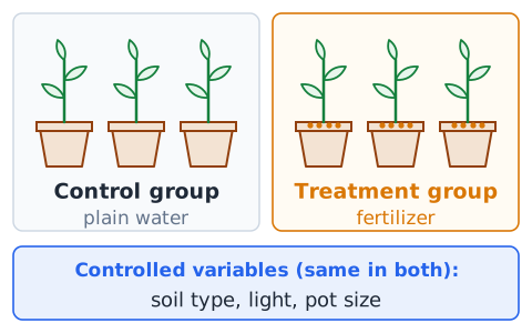
A control group is a set of subjects that does not receive the treatment being tested, so it serves as a baseline for comparison. Controlled variables are factors held constant across all groups. In a fertilizer test, plants given plain water are the control group, while soil type, light and pot size are controlled variables. You compare the treatment group with the control group to see the treatment's effect.

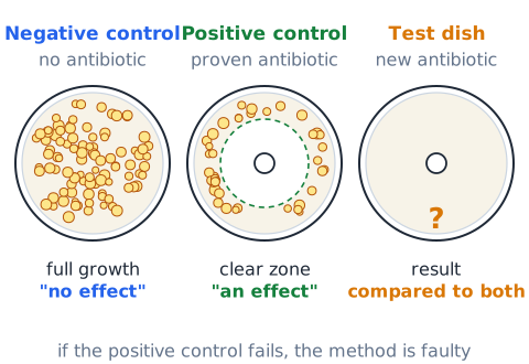
A negative control is a group expected to show no effect, such as a dish with no antibiotic in a test of bacterial growth. It shows what happens without the treatment and helps reveal contamination. A positive control uses something already known to work, such as a proven antibiotic. If the positive control fails, the method itself may be faulty. Together they show that the experiment can detect both "no effect" and "an effect."

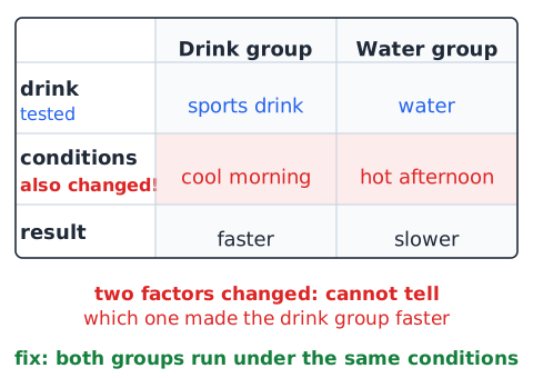
A confounding variable is a second factor that changes along with the independent variable and could also affect the result. If a cleaning test uses detergent A on cotton and detergent B on wool, fabric type is a confounder. When two factors change at once, you cannot tell which one caused the difference. The fix is to keep everything except the tested factor the same.

Random assignment means using chance, such as drawing names, to decide which subjects get the treatment. It spreads hidden differences, like plant health or a person's habits, evenly between groups so they do not favor one side. Random selection means choosing the sample from a population by chance so the sample represents that population. Assignment protects fairness inside the study; selection helps results apply more widely.

Replication means testing many subjects or running the experiment several times. One plant per group is risky because a single plant might be unusually weak or strong. Using ten or twenty independent plants per group lets you see whether a difference is consistent or just chance. Larger samples generally give more reliable averages. Measuring one plant twelve times does not equal twelve plants; it only checks your reading of that single plant.

A result is reproducible when other researchers following the same method get similar results. A hypothesis is falsifiable when some possible observation could show it to be wrong; "this metal expands when heated" could fail a test, so it is falsifiable. When new evidence conflicts with an accepted idea, scientists revise or replace the idea. Science builds confidence through repeated testing, not through a single proof.

Observer bias happens when what a researcher expects influences what the researcher records. In a blind study, the people measuring results do not know which subjects got the treatment. In a double-blind study, neither the subjects nor the researchers know. For example, a person scoring leaf damage without knowing which plants were sprayed is less likely to see what they hope to see.

In everyday speech, "theory" can mean a hunch. In science, a theory is a well-tested explanation that ties together many observations and has survived repeated attempts to disprove it, such as the theory of plate tectonics. A scientific law describes a pattern, often as an equation, while a theory explains why the pattern happens. Both can be refined if new evidence demands it.

A measurement has two parts: a number and a unit. Saying a board is "3 long" is meaningless; 3 m and 3 cm differ by a factor of 100. You can think of a quantity as

so 2.5 kg means 2.5 times one kilogram. Always carry units through calculations and write them with the answer.

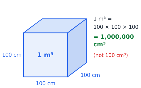
Science uses the metric system, built on the International System of Units (SI). The base units most often seen on the test are the meter (m) for length, the kilogram (kg) for mass, the second (s) for time, the kelvin (K) for temperature, and the ampere (A) for electric current. The liter (L) is a common volume unit; 1 L equals 1,000 cubic centimeters. Other units, such as newtons, are built from these.

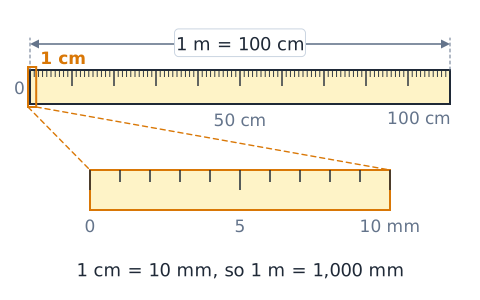
Metric prefixes multiply a unit by a power of ten. Kilo (k) means 1,000, so 1 km = 1,000 m. Centi (c) means one hundredth, so 1 m = 100 cm. Milli (m) means one thousandth, so 1 L = 1,000 mL and 1 g = 1,000 mg. Converting means moving the decimal point.

Micro, written with the Greek letter µ, means one millionth: 1 µm = 0.000001 m, and 1 m = 1,000,000 µm. Capital letters matter. Lowercase m is milli, but capital M is mega, or one million. So 5 mm is five millimeters, while 5 Mm is five million meters.

A conversion factor is a fraction equal to one, such as 60 min over 1 h. Multiply by it so the unit you have cancels and the unit you want remains:

If units do not cancel, flip the fraction.

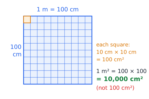
When a unit is squared or cubed, the conversion factor must be too. Since 1 m = 100 cm:

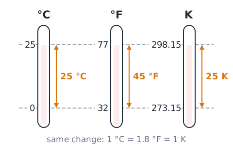
To convert a temperature reading from Celsius to Fahrenheit, use

so 25 °C is 77 °F. Kelvin is

For a change in temperature, the 32 offset drops out: a change of 1 °C equals a change of 1.8 °F, and equals a change of 1 K.

Density is mass per unit volume:

where $\rho$ (rho) is density, m is mass in grams and V is volume in cubic centimeters or milliliters. A block of 54 g that fills 20 cm³ has density 2.7 g/cm³. Water is about 1 g/mL; denser objects sink in it.

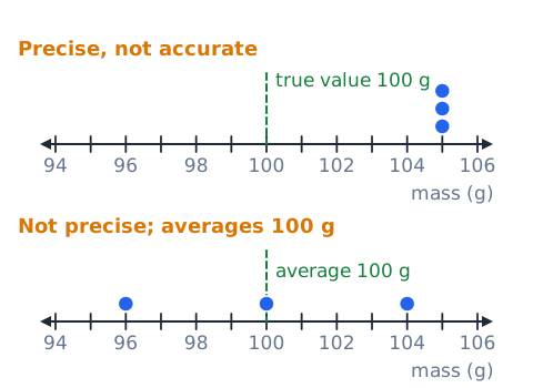
Accuracy describes how close a measurement is to the true value. Precision describes how close repeated measurements are to each other. A scale that reads 105 g three times for a 100 g standard is precise but not accurate. A scale that reads 96 g, 104 g and 100 g averages near the true value but is not precise. The goal is both: readings that cluster tightly around the true value.

Systematic error shifts every reading in the same direction, such as a scale that always reads 5 g high or a thermometer that is miscalibrated. Averaging more readings does not remove it; recalibrating does. Random error makes readings scatter unpredictably above and below the true value, perhaps from small hand movements or drafts. Repeating measurements and averaging reduces the effect of random error.

Resolution is the smallest change an instrument can show. A ruler marked in millimeters has a resolution of 1 mm, so a reading like 43 mm is reasonable, but 43.27 mm is not. Every measurement has some uncertainty, which can be written as a range, such as 43 mm plus or minus 1 mm. Report values only as finely as your instrument and method can support.

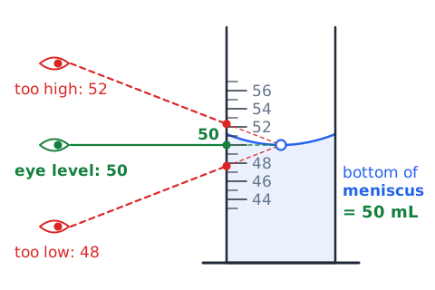
Parallax error happens when you read a scale from an angle, so the pointer or liquid level seems to line up with the wrong mark. To avoid it, put your eye level with the mark. When reading liquid in a graduated cylinder, look straight across at the bottom of the curved surface, called the meniscus (for water and most liquids). Reading from above or below makes the value look wrong.

Significant figures show how precise a value is. A calculated answer should not look more precise than the measurements used to make it. If a sample has a mass of 12.3 g and a volume of 4.7 mL, a calculator gives a density of 2.6170213 g/mL, but the data only justify two significant figures, so report 2.6 g/mL. Extra digits do not add accuracy; they only suggest precision you do not have.

Qualitative data describe qualities with words: color, smell, texture, or whether a reaction fizzed. Quantitative data use numbers with units: 23 °C, 4.5 cm, 12 seconds. Both are useful. "The solution turned blue" is qualitative; "the solution reached pH 8.2" is quantitative. Quantitative data allow calculations and precise comparisons, while qualitative notes can capture changes that are hard to measure.

An independent trial is a separate run of the experiment with its own setup, such as a different plant or a fresh batch of solution. A repeated reading measures the same subject again. Reading one thermometer three times checks your reading; testing three separate cups of water checks the result. Only independent trials show whether an outcome holds up across different subjects.

Before reading the numbers in a data table, read the title, the column headings and the units. A column labeled "Mass (g)" is very different from one labeled "Mass (kg)." Usually the independent variable is in the first column and the dependent variable in the next. Knowing what each column means prevents simple but costly mistakes.

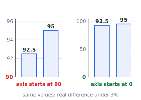
A line graph shows how one quantity changes as another changes, often over time. The horizontal axis (x-axis) usually shows the independent variable, such as time in seconds, and the vertical axis (y-axis) shows the dependent variable, such as distance in meters. Always check each axis label, its units and its scale. An axis that starts at 50 instead of 0, or that skips values, can make changes look larger or smaller than they really are.

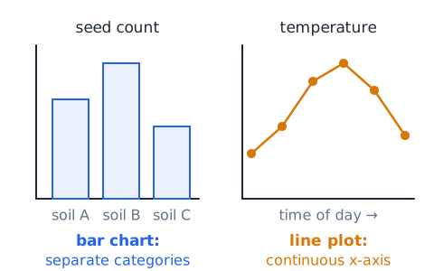
Bar charts compare separate categories, such as rainfall in four different cities or seed counts for three soil types. Line plots connect points to show change across a continuous variable, such as temperature through a day. Use a line when the x-axis values are in order and in-between values make sense. Do not read a trend between bars for unrelated categories.

A bar's height is meaningful only relative to the baseline. If the vertical axis starts at 90 instead of 0, a bar at 95 may look twice as tall as a bar at 92.5, even though the real difference is under 3 percent. Read the actual values from the axis rather than comparing bar sizes by eye.

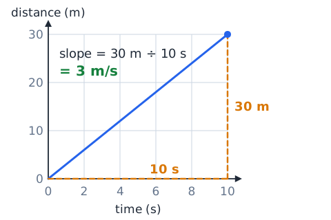
On a line graph, slope is the change in the vertical quantity divided by the change in the horizontal quantity. On a distance-time graph, slope is speed: if distance goes from 0 m to 30 m while time goes from 0 s to 10 s, the speed is 3 m/s. A steeper line means a faster rate; a downward slope means the quantity is decreasing.

An average rate uses only the starting and ending values:

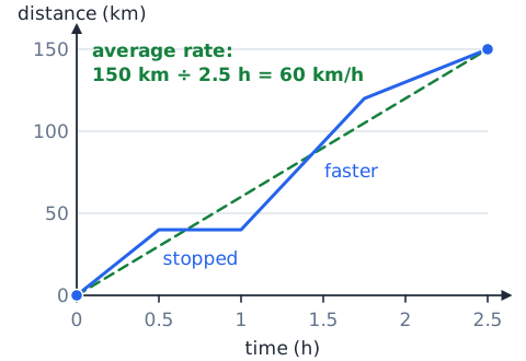
where $\Delta$ means "change in." A car that covers 150 km in 2.5 h averages 60 km/h, even if it sometimes stopped and sometimes went faster. The instantaneous rate is the rate at one moment, like a speedometer reading, and can differ from the average.

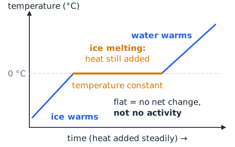
A flat section on a graph means the measured quantity is not changing, but processes may still be happening. When ice melts, its temperature stays at 0 °C while heat is still being added; the energy goes into melting instead of warming. A steady room temperature may reflect heating and cooling balancing out. A flat line shows no net change, not necessarily no activity.

The mean is the sum of the values divided by how many there are. The median is the middle value after sorting. The range is the largest value minus the smallest. For 2, 5, 5, 8 and 10: the mean is 30 divided by 5, or 6; the median is 5; the range is 10 minus 2, or 8.

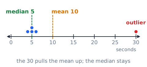
An outlier is a value far from the rest. In a set of reaction times of 4, 5, 5, 6 and 30 seconds, 30 is an outlier. It pulls the mean up to 10 seconds, while the median stays at 5. Do not simply delete outliers: check whether one came from a recording mistake or equipment problem. If it is real, report it and consider using the median.

Percent change equals the change divided by the original value, times 100. The original value is the reference. Going from 50 to 40 is a 10-unit drop, which is 20% of 50, so a 20% decrease. Going from 40 back to 50 is a 10-unit rise, which is 25% of 40, so a 25% increase. Same difference, different reference, different percent.

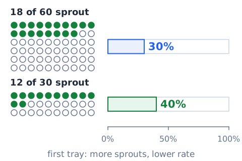
Raw counts can mislead when groups differ in size. Normalizing means turning counts into a common basis, such as a percent or a rate per 1,000. If 18 of 60 seeds sprout in one tray and 12 of 30 in another, the first tray has more sprouts, but its germination rate is 30% versus 40% for the second. The smaller tray did proportionally better.

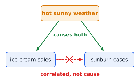
Two quantities are correlated when they tend to change together. That alone does not show that one causes the other. Ice cream sales and sunburn cases both rise in summer, but ice cream does not cause sunburn; a third factor, hot sunny weather, drives both. Causation needs a controlled experiment or strong additional evidence that rules out other explanations.

Some questions cannot be tested with a controlled experiment. Scientists cannot ethically expose people to a harmful substance to see whether it causes disease, and they cannot assign earthquakes to some cities and not others. In these cases they use observational studies, comparing groups that already differ, along with careful statistics. Such studies can reveal strong associations, but conclusions about cause are made with more caution.

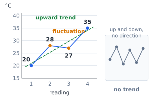
A trend is an overall direction in data over time, upward or downward. Fluctuation is short-term up-and-down movement around that direction. Readings of 20, 28, 27 and 35 °C show an upward trend with one small dip. If values bounce up and down with no overall direction, there is no trend. Look at the whole data set before describing it, not at a single interval.

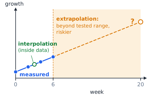
Interpolation estimates a value between measured points, such as estimating a temperature at minute 3 from readings at minutes 2 and 4. It is usually fairly safe. Extrapolation estimates beyond the measured range, such as predicting growth at week 20 from data that stop at week 6. Extrapolation is riskier because conditions may change outside the range you tested.

To compare groups of different sizes, divide by a fair denominator. A town of 4,000 people with 12 cases and a city of 10,000 with 15 cases compare this way:

The town has the higher rate per 1,000 people.

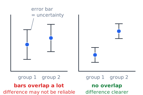
Error bars are lines drawn above and below a plotted point to show uncertainty or spread in the data. If the error bars of two groups overlap a lot, the difference between their averages may not be reliable. Many simple graphs show only averages without error bars or sample sizes. In that case you can describe the difference in averages, but you cannot judge how trustworthy it is.

A real prediction is made before the data are collected, so the result can confirm or contradict it. Post-hoc storytelling invents an explanation after seeing the results, and almost any result can be explained that way. Suppose a researcher sees that one plant grew taller and only then decides it was due to the pot's color. That idea was not tested; it needs a new experiment designed to check it.

A conclusion should stay within the conditions that were tested. If an experiment used one species of bean, at room temperature, for three weeks, the result applies to those conditions. Claiming it holds for all plants, all climates or all time spans goes beyond the evidence. Good conclusions use phrases like "under these conditions" or "in this sample."

Before accepting a claim, ask: What was measured, and in what units? Was only one factor changed? Was there a control group? How many independent trials or subjects were there? Do the numbers actually show the change claimed, after reading the axes and baselines? Does the conclusion stay within the conditions tested? Could another factor explain the result? A strong claim passes all of these checks.

Read the last line of the question first so you know what is being asked: a variable, a unit, a calculation or a conclusion. Then read the details and underline numbers and units mentally. For calculations, estimate the size of the answer before checking choices. For design questions, look for the one factor that changed. For conclusions, prefer the choice that is supported and limited, not sweeping.

Cross out choices with absolute words like always, never, proves or all when the data come from a few trials. Also watch for direction reversals: a choice that says the dependent variable caused the independent variable, or that a quantity decreased when it rose. Once those are gone, the remaining choice is usually the careful, data-matched one.

The ASVAB does not allow a calculator, so use shortcuts. For metric conversions, shift the decimal: 0.36 L becomes 360 mL by moving it three places right. For a graph slope, choose two points on grid lines. If a line passes through 0 s, 0 m and 8 s, 40 m:

Watch for these errors. Mixing up the independent and dependent variables. Calling a controlled variable a control group. Changing two factors at once. Treating repeated readings of one subject as separate trials. Confusing precision with accuracy. Dropping units or prefixes. Converting area with a factor of 100 instead of 10,000. Adding the 32 offset to a temperature change. Comparing raw counts from groups of different sizes. Using the wrong reference for percent change. Reading bars without checking the baseline. Claiming causation from correlation.

Scenario: A student wants to know whether light color affects how fast radish seedlings grow. Step one: the independent variable is light color, such as red, blue and white. Step two: the dependent variable is seedling height after ten days. Step three: control seed type, soil, water, temperature, light brightness and hours of light. Step four: use at least ten seedlings per color and assign them at random. Answer: this design changes only the light color, so differences in height can be linked to it.

Scenario: A coach tests whether a sports drink improves sprint times. Runners who drink it run in the cool morning; runners who drink water run in the hot afternoon. The drink group is faster. Step one: the independent variable is the drink. Step two: temperature and time of day also changed with it. Answer: temperature is a confounding variable, so the test cannot show that the drink caused faster times. Both groups should run under the same conditions.

Problem: A pill contains 750 mg of an ingredient. How many grams is that? Step one: 1 g = 1,000 mg. Step two: dividing by 1,000 moves the decimal three places left. Answer: 750 mg equals 0.75 g.

Problem: A tabletop is 0.4 m². Express it in cm². Since 1 m² = 10,000 cm²:

Answer: 4,000 cm², not 40 cm².

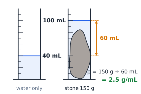
Problem: A stone of mass 150 g is lowered into a cylinder, and the water level rises from 40 mL to 100 mL. Find its density. The volume is 100 minus 40, or 60 mL.

The stone is denser than water, so it sinks.

Problem: A tank's water level is 10 cm at 0 h, 13 cm at 2 h, 16 cm at 4 h and 19 cm at 6 h. Find the rate.

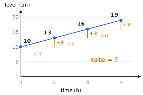
Each 2-hour step adds 3 cm, which agrees.

Problem: Readings are 3, 8, 4, 12 and 8. Sorted: 3, 4, 8, 8, 12, so the median is 8.

The mean and median differ because the 12 pulls the mean.

Problem: Pump A moves 450 L in 15 min. Pump B moves 600 L in 25 min. Which pump is faster?

Pump B moved more water in total, but Pump A is faster.

Problem: A plant grows from 25 cm to 32 cm. Find the percent increase. The change is 7 cm, and the original is 25 cm.

Answer: a 28% increase.

Scenario: A lab tests a new coating on five steel plates kept in a humid room for one month. None rust, while three of five uncoated plates do. Which conclusion is best? Step one: the coating appears to reduce rust under these conditions. Step two: the sample is small, the time is short, and only humidity was tested. Answer: the coating reduced rust in this trial, and larger, longer tests in other conditions, such as salt spray, are needed before claiming it prevents rust everywhere.

Scenario: A thermometer placed in boiling water at sea level reads 97.0, 97.1 and 97.0 °C. Pure water boils at about 100 °C there. Step one: the readings are tightly clustered, so precision is good. Step two: they are about 3 °C low every time, which is a systematic error. Answer: the thermometer is precise but inaccurate and should be recalibrated; averaging more readings would not fix it.

Problem: Water warms from 15 °C to 40 °C. What is the change in °F? The change is 25 °C, and the offset does not apply to a difference.

Check: 59 °F to 104 °F is also a 45 °F rise.

Setup: A student adds 0, 5 or 10 g of salt to equal cups of water and times how long each takes to boil on the same burner.

Prompt: Independent variable? Answer: amount of salt.

Prompt: Dependent variable? Answer: time to boil.

Prompt: Name two controlled variables. Answer: water volume and burner setting.

Prompt: If the student tests 25 cups in all and 15 boil within 8 minutes, what percent is that? Answer:

Setup: A gardener tests a mulch by using it on the sunny side of a yard and not on the shady side.

Prompt: What is wrong? Answer: sunlight changes along with mulch, so it is a confounder.

Prompt: How should it be improved? Answer: use several beds with matching sun and soil, and randomly choose which beds get mulch.

Prompt: 4.2 km to meters. Answer: 4,200 m.

Prompt: 35 mm to centimeters. Answer: 3.5 cm.

Prompt: 1,800 mL to liters. Answer: 1.8 L.

Prompt: 0.09 kg to grams. Answer: 90 g.

Setup: Plant heights over four weeks are 12, 18, 15 and 22 cm.

Prompt: Did height rise every week? Answer: No, it dropped in week three.

Prompt: Overall change? Answer: up 10 cm, from 12 to 22 cm.

Prompt: Best description? Answer: an overall rise with one dip.

Setup: A report notes that cities with more bike lanes have fewer traffic deaths and concludes that bike lanes cause safer roads.

Prompt: What kind of evidence is this? Answer: correlation from observation.

Prompt: What else could explain it? Answer: those cities may also have lower speed limits or more public transit. The claim needs a study that accounts for such factors.

Prompt: A balance reads 2 g high every time. Which error is this? Answer: systematic; recalibrate or subtract 2 g.

Prompt: Stopwatch times for one falling ball are 1.21, 1.18 and 1.24 s. Which error causes the spread? Answer: random, mainly reaction time; average several trials.

A hypothesis is a testable explanation, and a prediction is the result it leads you to expect. Change one independent variable, measure the dependent variable, and hold controlled variables constant. Use a control group, random assignment and many independent trials. Carry units, use metric prefixes correctly, and square or cube conversion factors for area and volume. Precision is repeatability; accuracy is closeness to the true value. Compare rates and percents, not raw totals. Correlation is not causation, and conclusions should stay within the conditions tested.